[PaperReading] Color Transfer between Images, Erik Reinhard et al, 2001

Implementation and improvement of paper: Color Transfer between Images, Erik Reinhard et al, 2001 —— A simple statistical analysis to impose one image’s color characteristics on another.

I put forward a method called PureColorGuidedStyle which is a easier, faster more controllable version based on this paper’s method. It can obtain better results most of the time.

★Source codes and images here

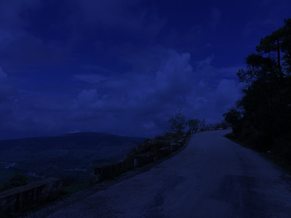
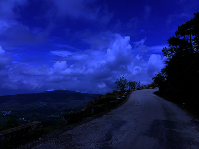
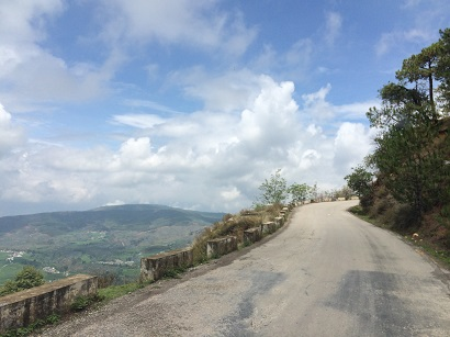
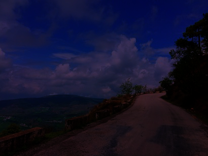
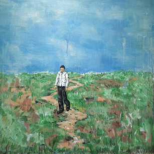
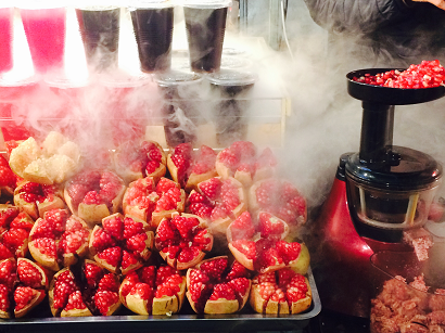
All photos except dress for girl are taken by myself. Feel free to take away if you like.
For the paper’s method, each group of images is aligned in a row. From left to right are source image, result image and right image respectively.
Result image is obtained by imposing target image’s color characteristics on source image.

For PureColorGuidedStyle method, each group of images is arranged in two rows. First row from left to right are source image, result image with a smaller scale value and result image with a bigger scale value respectively. The second row is the pure color target image.
Result image is obtained by imposing target color on source image. Adjust effect by tuning the scale value.

---

Intuition

Decorrelated color space

Choose an orthogonal color space without correlations between the axes to simplify color modification process: Ruderman et al.’s perception-based color space lαβ minimizes correlation between channels for many natural scenes. Additionally, this color space is logarithmic, which means to a first approximation that uniform changes in channel intensity tend to be equally detectable. This space is based on data-driven human perception research that assumes the human visual system is ideally suited for processing natural scenes.

Statistics and color correction

Make a synthetic image take on another image’s look and feel. Some aspects of the distribution of data points in lαβ space to transfer between images: the mean and standard deviations along each of the three axes suffice.
The result’s quality depends on the images’ similarity in composition. Sometimes fail: Manually select two or more pairs of clusters in lαβ space for transformation. Another possible extension would be to compute higher moments such as skew and kurtosis, which are respective measures of the lopsidedness of a distribution and of the thickness of a distribution’s tails. Imposing such higher moments on a second image would shape its distribution of pixel values along each axis to more closely resemble the corresponding distribution in the first image.

Algorithm

Normal without color correction

• RGB -> lαβ Converting RGB signals to Ruderman et al.’s perception-based color space lαβ.

  • RGB -> LMS. Combining the following two matrices gives the following transformation between RGB and LMS cone space:
    $$
    \begin{bmatrix}L \cr M \cr S \cr \end{bmatrix} =
    \begin{bmatrix}0.3811 & 0.5783 & 0.0402 \cr 0.1967 & 0.7244 & 0.0782 \cr 0.0241 & 0.1228 & 0.8444 \cr \end{bmatrix}
    \begin{bmatrix}R \cr G \cr B \cr \end{bmatrix}
    $$
    • RGB -> XYZ
      $$
      \begin{bmatrix}X \cr Y \cr Z \cr \end{bmatrix} =
      \begin{bmatrix}0.5141 & 0.3239 & 0.1604 \cr 0.2651 & 0.6702 & 0.0641 \cr 0.0241 & 0.1228 & 0.8444 \cr \end{bmatrix}
      \begin{bmatrix}R \cr G \cr B \cr \end{bmatrix}
      $$
    • XYZ -> LMS
      $$
      \begin{bmatrix}L \cr M \cr S \cr \end{bmatrix} =
      \begin{bmatrix}0.3897 & 0.6890 & 0.0787 \cr -0.2298 & 1.1834 & 0.0464 \cr 0.0000 & 0.0000 & 1.0000 \cr \end{bmatrix}
      \begin{bmatrix}X \cr Y \cr Z \cr \end{bmatrix}
      $$
  • Convert the data to logarithmic space to eliminate skew.
    $$
    L = logL \\
    M = logM \\
    S = logS
    $$
  • LMS -> lαβ
    $$
    \begin{bmatrix}l \cr α \cr β \cr \end{bmatrix} =
    \begin{bmatrix}\frac{1}{\sqrt 3} & 0 & 0 \cr 0 & \frac{1}{\sqrt 6} & 0 \cr 0 & 0 & \frac{1}{\sqrt 2} \cr \end{bmatrix}
    \begin{bmatrix}1 & 1 & 1 \cr 1 & 1 & -2 \cr 1 & -1 & 0 \cr \end{bmatrix}
    \begin{bmatrix}L \cr M \cr S \cr \end{bmatrix} =
    \begin{bmatrix}\frac{1}{\sqrt 3} & \frac{1}{\sqrt 3} & \frac{1}{\sqrt 3} \cr \frac{1}{\sqrt 6} & \frac{1}{\sqrt 6} & \frac{-2}{\sqrt 6} \cr \frac{1}{\sqrt 2} & \frac{-1}{\sqrt 2} & 0 \cr \end{bmatrix}
    \begin{bmatrix}L \cr M \cr S \cr \end{bmatrix}
    $$

• Color processing(Statistics and color correction) Make a synthetic image take on another image’s look and feel. More formally this means that we would like some aspects of the distribution of data points in lαβ space to transfer between images.

  • Compute the means and standard deviations for each axis(3 in total) separately in lαβ space
  • Subtract the mean from the data points
    $$
    l^{\ast} = l - \langle l_s \rangle \\
    α^{\ast} = α - \langle α_s \rangle \\
    β^{\ast} = β - \langle β_s \rangle
    $$
  • scale the data points comprising the synthetic image by factors determined by the respective standard deviations:
    $$
    l^{‘} = {\sigma_t^l \over \sigma_s^l} l^{\ast} \\
    α^{‘} = {\sigma_t^\alpha \over \sigma_s^\alpha} α^{\ast} \\
    β^{‘} = {\sigma_t^\beta \over \sigma_s^\beta} β^{\ast}
    $$
  • Add the averages computed for the photograph
    $$
    l^{‘’} = l^{‘} + \langle l_t \rangle \\
    α^{‘’} = α^{‘} + \langle α_t \rangle \\
    β^{‘’} = β^{‘} + \langle β_t \rangle
    $$
• lαβ -> RGB Transfer result in lαβ to RGB to display it.
  • lαβ -> LMS
    $$
    \begin{bmatrix}L \cr M \cr S \cr \end{bmatrix} =
    \begin{bmatrix}1 & 1 & 1 \cr 1 & 1 & -1 \cr 1 & -2 & 0 \cr \end{bmatrix}
    \begin{bmatrix}\frac{1}{\sqrt 3} & 0 & 0 \cr 0 & \frac{1}{\sqrt 6} & 0 \cr 0 & 0 & \frac{1}{\sqrt 2} \cr \end{bmatrix}
    \begin{bmatrix}l \cr α \cr β \cr \end{bmatrix} =
    \begin{bmatrix}\frac{1}{\sqrt 3} & \frac{1}{\sqrt 6} & \frac{1}{\sqrt 2} \cr \frac{1}{\sqrt 3} & \frac{1}{\sqrt 6} & \frac{-1}{\sqrt 2} \cr \frac{1}{\sqrt 3} & \frac{2}{\sqrt 6} & 0 \cr \end{bmatrix}
    \begin{bmatrix}l \cr α \cr β \cr \end{bmatrix}
    $$
  • Raising the pixel values to the power ten to go back to linear space.
    $$
    L = L^{10} \\
    M = M^{10} \\
    S = S^{10}
    $$
  • LMS -> RGB
    $$
    \begin{bmatrix}R \cr G \cr B \cr \end{bmatrix} =
    \begin{bmatrix}4.4679 & -3.5873 & 0.1193 \cr -1.2186 & 2.3809 & -0.1624 \cr 0.0497 & 0.2439 & 1.2045 \cr \end{bmatrix}
    \begin{bmatrix}L \cr M \cr S \cr \end{bmatrix}
    $$

Color correction

Example: If the synthetic image contains much grass and the photograph has more sky in it, then we can expect the transfer of statistics to fail.

• Select separate swatches of grass and sky and compute their statistics, leading to two pairs of clusters in lαβ space (one pair for the grass and sky swatches).
• Convert the whole rendering to lαβ space.
• Scale and shift each pixel in the input image according to the statistics associated with each of the cluster pairs.
• Compute the distance to the center of each of the source clusters and divide it by the cluster’s standard deviation $\sigma_{c,s}$. This division is required to compensate for different cluster sizes.
• Blend the scaled and shifted pixels with weights inversely proportional
  to these normalized distances, yielding the final color.

Implementation

Implement with The CImg Library in C++ language. Test on Visual Studio 2015, C++11. Images should be of bmp format (much easier to convert by ImageMagick).
But for first understanding of the algorithm, I recommend reading this MATLAB version written by hangong if you are familiar with MATLAB.

RGB -> lαβ color space

<=> RGB -> LMS -> logarithmic space -> lαβ color space

CImg<float> RGB2Lab(CImg<unsigned int> RGBimg) {
    if (RGBimg._spectrum != 3) { // Number of colour channels
        cerr << "RGB2Lab(): Instance is not a RGB image." << endl;
    }
    CImg<float> Labimg(RGBimg._width, RGBimg._height, 1, 3, 0); // w,h,depth,spectrum,initVal
    float R, G, B, L, M, S, l, alpha, beta;
    cimg_forXY(RGBimg, x, y) {
        R = cimg::max(1.0 * RGBimg(x, y, 0) / 255, 1.0 / 255); // must be 1.0f, or 1/255 will be zero!!
        G = cimg::max(1.0 * RGBimg(x, y, 1) / 255, 1.0 / 255);
        B = cimg::max(1.0 * RGBimg(x, y, 2) / 255, 1.0 / 255);

        // RGB -> LMS
        L = 0.3811f*R + 0.5783f*G + 0.0402f*B;
        M = 0.1967f*R + 0.7244f*G + 0.0782f*B;
        S = 0.0241f*R + 0.1288f*G + 0.8444f*B;
        // Convert the data to logarithmic space
        L = log10(L); // log(x), x > 0
        M = log10(M);
        S = log10(S);
        // LMS -> Lab
        l = 1.0 / sqrt(3)*L + 1.0 / sqrt(3)*M + 1.0 / sqrt(3)*S;
        alpha = 1.0 / sqrt(6)*L + 1.0 / sqrt(6)*M - 2 / sqrt(6)*S;
        beta = 1.0 / sqrt(2)*L - 1.0 / sqrt(2)*M + 0 * S;

        Labimg(x, y, 0) = l;
        Labimg(x, y, 1) = alpha;
        Labimg(x, y, 2) = beta;
    }
    return Labimg;
}

Color processing(Statistics and color correction)

In function CImg<float> transferOfStatistics(CImg<float> Lab_source, CImg<float> Lab_target), we impose Lab_target image’s color characteristics on Lab_source and obtain Lab_result image in the following steps.

• Compute the means and standard deviations for each axis separately in lαβ space of Lab_source and Lab_target.

unsigned long n_source = Lab_source._width * Lab_source._height;
cimg_forXYC(Lab_source, x, y, c)
    mean_source(c) += Lab_source(x, y, c);
cimg_forX(mean_source, c)
    mean_source(c) /= n_source;
cimg_forXYC(Lab_source, x, y, c)
    std_source(c) += pow(Lab_source(x, y, c) - mean_source(c), 2.0);
cimg_forX(mean_source, c)
    std_source(c) = sqrt(std_source(c) / n_source);

• Transfer by adjust the mean and standard deviations along each of the three axes: firstly subtract the mean from the data points, and then scale the data points comprising the synthetic image by factors determined by the respective standard deviations, finally add the averages computed for the photograph.

cimg_forXYC(Lab_source, x, y, c) {
    Lab_result(x, y, c) = Lab_source(x, y, c) - mean_source(c);
    Lab_result(x, y, c) = Lab_result(x, y, c) * (std_target(c) / std_source(c));
    Lab_result(x, y, c) = Lab_result(x, y, c) + mean_target(c);
}

For PureColorGuidedStyle method, the second equation is changed to

/* PureColorGuidedStyle method: Input a pure color target image and tune the 
*  scale value to get a result image more conveniently and controllable. */
float scale_val = 4;
Lab_result(x, y, c) = Lab_result(x, y, c) * scale_val;

lαβ -> RGB color space

Function CImg<unsigned int> Lab2RGB(CImg<float> Labimg) is the inverse process of CImg<float> RGB2Lab(CImg<unsigned int> RGBimg)

• lαβ -> LMS

  L = sqrt(3.0) / 3.0 * l + sqrt(6) / 6.0 * alpha + sqrt(2) / 2.0 * beta;
  M = sqrt(3.0) / 3.0 * l + sqrt(6) / 6.0 * alpha - sqrt(2) / 2.0 * beta;
  S = sqrt(3.0) / 3.0 * l - sqrt(6) / 3.0 * alpha - 0 * beta;

• Raising the pixel values to the power ten to go back to linear space.

  L = pow(10.0, L);
  M = pow(10.0, M);
  S = pow(10.0, S);

• LMS -> RGB

  R = 4.4679*L - 3.5873*M + 0.1193*S;
  G = -1.2186*L + 2.3809*M - 0.1624*S;
  B = 0.0497*L - 0.2439*M + 1.2045*S;

Results

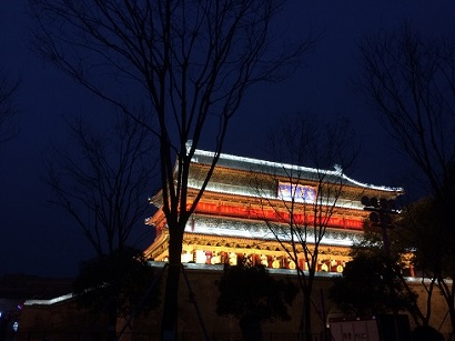
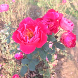
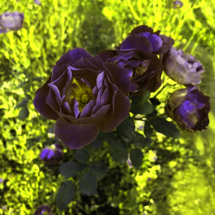
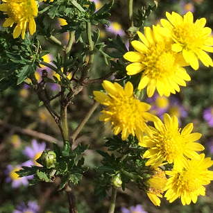
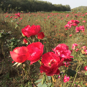
From left to right are source image, result image and target respectively each row. Result image is obtained by imposing source image’s color characteristics on target image.

Favorable results

Results are favorable when you want to change the source image’s style in whole similar to the main color style of target image.

Undesirable Results

We can notice that what this algorithm doing is extracting a color from target image and then cover a monochrome layer of this color to the source image. It’s simple and favorable for some images. But never expect it can automatically recolor even if they have the same composition!

If you want to recolor the dress only, my first thought is to perform edge detection and exclude the background out of the process domain. But it’s not about Color Transfer. So forget it.

---

And note that the final color of result image is a combination of source image’s color and the monochrome color extracted from target image. So sometimes the result’s color is totally different from target image. For example, you may expect the pink flower change to yellow style but their combination is purple.

In the extreme case, the target image has pure color and you got a same pure color result image no matter what the source image is. This is because the standard deviation of target image $\sigma_t$ is zero. The target iamge(which has shifted by its own mean) is scale by ${\sigma_t \over \sigma_s}$ and then shift by mean of target image. So the result is mean of target image which is pure color.

My Improvement(PureColorGuidedStyle)

We can easily remedy this issue. Just manually set a scale value in place of ${\sigma_t \over \sigma_s}$.

$$
l^{‘} = \max(scale_v, {\sigma_t^l \over \sigma_s^l}) l^{\ast} \\
α^{‘} = \max(scale_v, {\sigma_t^\alpha \over \sigma_s^\alpha}) α^{\ast} \\
β^{‘} = \max(scale_v, {\sigma_t^\beta \over \sigma_s^\beta}) β^{\ast}
$$

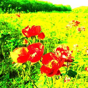
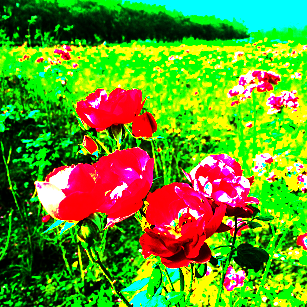
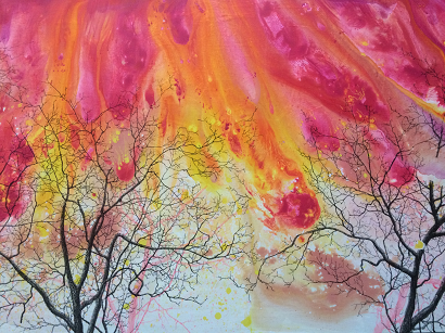
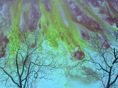
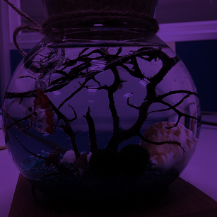
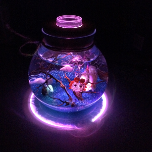
I set value 2 and 4 respectively for this example and got red flowers in yellow and green background. The scale value means you want to preserve(shrink or enlarge) the source image in what extent. A big value means the source image’s color counts a lot and it will combine with the target color. The smaller the value, the more similar the color is to the pure color. So its much more convenient and controllable to input a pure color target image and tune the scale value! I call it PureColorGuidedStyle method.
The pure color target image can be rather small(several pixels are enough) so it saves time. This method also saves you out of choosing target images while may get undesirable results. You can also change the style by tuning the scale value easily.

---

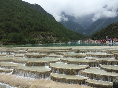
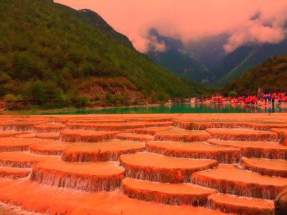
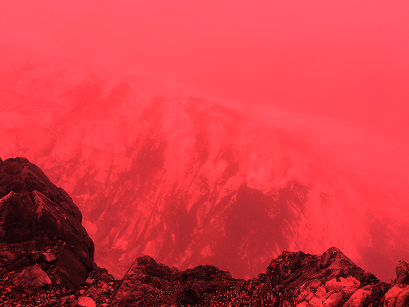
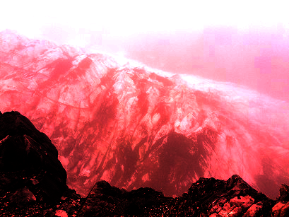
I also notice discontinuity will appear in some images.

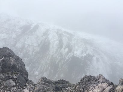
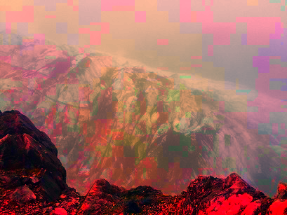
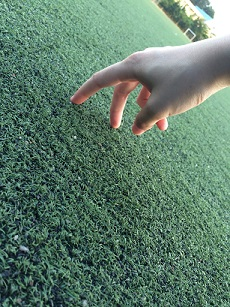
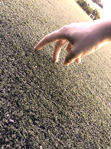
I don’t exactly know the reason but just try my PureColorGuidedStyle method and get the following results. The scale value for result images from left to right are 2 and 6 respectively. The discontinuity totally disappear and the snow mountain outbreak to a burning mountain!

---

In fact, the author of this paper gives a method for color correction by choosing an appropriate source image and apply its characteristic to another image. I am not going to implement it since it’s inconvenient to manually select and handle swatches.