Histogram equalization is a technique for adjusting image intensities to enhance contrast. In this post, I implement grayscale image histogram equalization and three methods of color image histogram equalization. Detail analyses and results are given.

Grayscale Image
Derivation
You are welcome to read my chinese version derivation of the process of implementing the histogram equalization operation and MATLAB version code. Or you can read this) more detailed and explictly explained derivation.
Following derivation without proof of transformation comes from Wikipedia:Histogram Equalization.
Consider a discrete grayscale image $\{x\}$ and let $n_i$ be the number of occurrences of gray level $i$. The probability of an occurrence of a pixel of level $i$ in the image is
$$ p_x(i)=p(x=i)=\frac {n_i}{n}, \quad 0 \leq i<L $$
$L$ being the total number of gray levels in the image (typically 256), $n$ being the total number of pixels in the image, and $p_{x}(i)$ being in fact the image’s histogram for pixel value $i$, normalized to $[0,1]$.
Let us also define the cumulative distribution function corresponding to $p_x$ as
$$cdf_x(i) = \sum_{j=0}^i p_x(j)$$
which is also the image’s accumulated normalized histogram.
We would like to create a transformation of the form $y = T(x)$ to produce a new image $\{y\}$, with a flat histogram. Such an image would have a linearized cumulative distribution function (CDF) across the value range, i.e.
$$ cdf_{y}(i)=iK$$
for some constant $K$. The properties of the CDF allow us to perform such a transform (see Inverse distribution function); it is defined as
$$ cdf_{y}(y^{\prime })=cdf_{y}(T(k))=cdf_{x}(k) $$
where k is in the range $[0,L]$. Notice that T maps the levels into the range $[0,1]$, since we used a normalized histogram of $\{x\}$. In order to map the values back into their original range, the following simple transformation needs to be applied on the result:
$$ y^{\prime }=y\cdot (\max\{x\}-\min\{x\})+\min\{x\} $$
Implementation
Implement with The CImg Library in C++ language. Test on Visual Studio 2015, C++11. Images should be of bmp format(much easier to convert by ImageMagick).
But for first understanding of the algorithm, I recommend reading my MATLAB version if you are familiar with MATLAB.
RGB to Grayscale
See the RGB to grayscale equation.
Suppose the RGB value of a color is (r, g, b), where r, g, and b are integers between 0 and 255. The grayscale weighted average, x, is given by the formula
$x = 0.299r + 0.587g + 0.114b$
Notice that the colors are not weighted equally. Since pure green is lighter than pure red and pure blue, it has a higher weight. Pure blue is the darkest of the three, so it receives the least weight.
|
|
Histogram Calculation
The total number of gray levels (number of possible intensity values) $L$ in the image is typically 256, so I use a $256 \times 1$ matrix histogram to store the occurrence of a pixel of level $i$ (haven’t normalized to $[0,1]$). $n_{r_j}$ is the number of pixels of level $r_j$. The image’s histogram for pixel value $i$ is
$$ histogram(i) = n_{r_j}, \quad 0 \leq i<L $$
|
|
Histogram Equalization
First get the input image’s histogram. And then calculate the cumulative distribution function corresponding to normalized histogram as
$$cdf(j) = \sum_{j=0}^k \frac{n_{r_j}}{n}$$
$n$ being the total number of pixels in the image.
Transform input image’s intensity $r_k$ into output image’s intensity $s_k$
$$ s_k = T(r_k) = round(cdf(r_k) \times (L-1)) $$
where round() rounds down to the nearest integer. Store $s_k$ into equalized array.
|
|
Finally we get histogram equalization result.
|
|
Color Image
The above describes histogram equalization on a grayscale image. However it can also be used on color images. Here’s three ways and their implementations.
Also see: my MATLAB version code and chinese version report.
Independent histogram equalization based on color channel
Implementation
Applying the grayscale image method separately to the Red, Green and Blue channels of the RGB color values of the image and rebuild an RGB image from the three processed channels.
|
|
Analysis
Disadvantage: Not considering the relevance of R, G and B channel but process then respectively will distort the image. See Wekipedia:
Applying the same method on the Red, Green, and Blue components of an RGB image may yield dramatic changes in the image’s color balance since the relative distributions of the color channels change as a result of applying the algorithm.
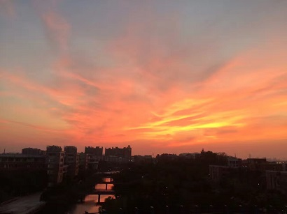
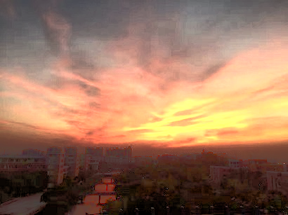
Advantage: It processes fastest out of these three method. And maybe we can use it for some special unrealistic effect like the sunset?
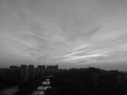
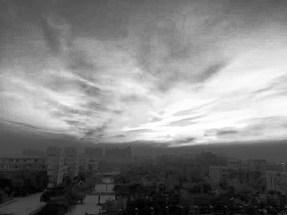
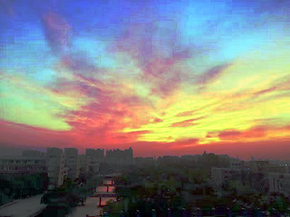
Here’s an example.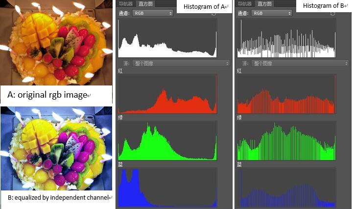
The R, G and B channel’s histogram are totally different. When we apply independent equalization on them respectively, we get B. The intensities have been better distributen on the histogram but B’s color is out of balance. This is caused by the change of relative distributions of the color channels. For example, A’s green components mostly distribute on low levels/small intensities while B’s green components distribute over the whole levels much more evenly. This makes B looks bluer.
Histogram equalization based on average value of color channel
What we want is a better distributed RGB histogram but not all histograms including color channels. So we can take the three channels as a whole when calculate the histogram.
Implementation
The only difference between the second and first method is that the second method uses an average histogram of the three channels’ histograms.
|
|
Analysis
This method considers the relevance of R, G and B channel and gets better results.
Here’s an example.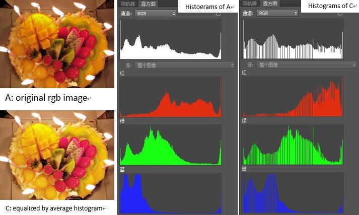
The RGB histogram is better distributed and the contrast increases. The histograms of R, G and B channels also spread out but still preserve the original relative distribution.
Intensity component equalization based on HSI color space
Implementation
The image is first converted to HSI color space, then apply the grayscale method to the luminance without resulting in changes to the hue and saturation of the image.
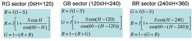
Converting colors from RGB to HSI
The formula I used comes from Digital Image Processing (3rd Edition): Rafael C. Gonzalez, Richard E.Woods, section 6.2.3 The HSI Color Model. Here I found the same formula from Yao Wang’s PPT for quick reference.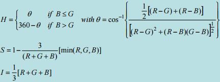
|
|
Perform histogram equalization on the intensity channel
|
|
Converting colors from HSI to RGB
|
|
Rebuild an RGB image from the three processed channels
|
|
Analysis
This method often get good results, but sometimes it may not. Here’s an example.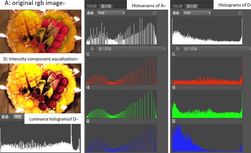
In image D, the mangos are too bright and the strawberries are too dark which hide the detail. This is caused by the uneven distribution of RGB histogram because equalization is on luminance channel of HSI color space.
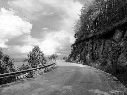
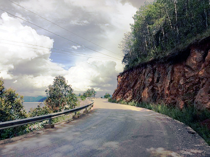
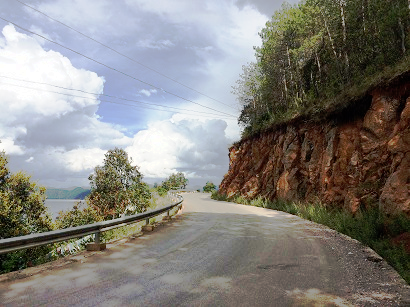
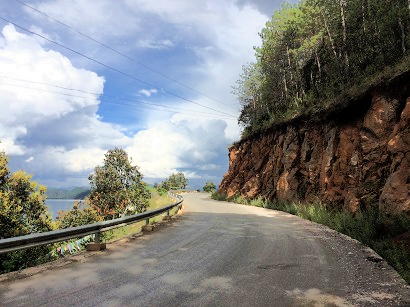
Results
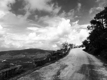
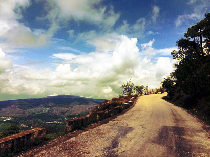
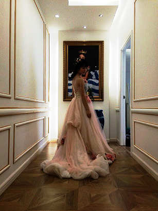
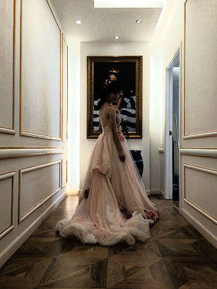
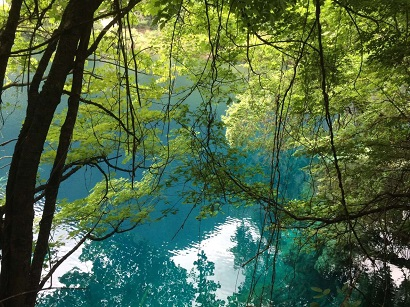
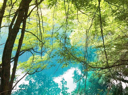
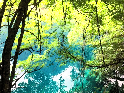
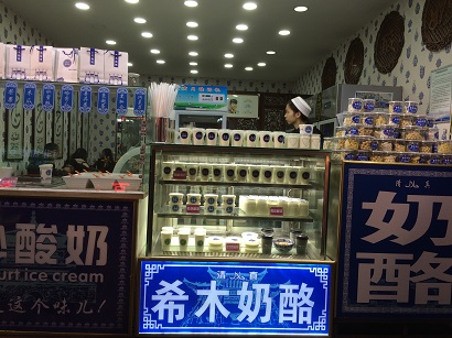
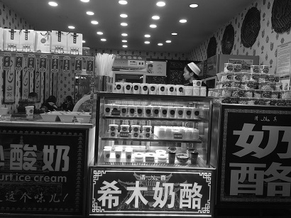
All photos are taken by myself. Feel free to take away if you like.
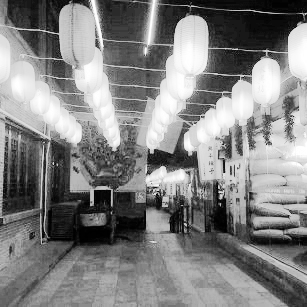
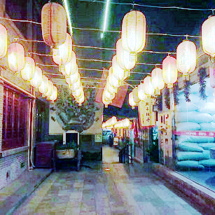
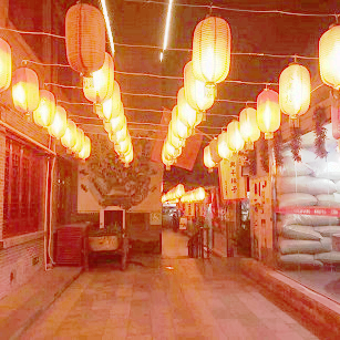
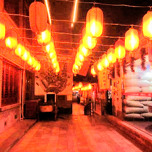
Each group of six images is arranged in two rows in the following order.
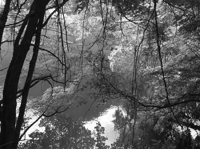
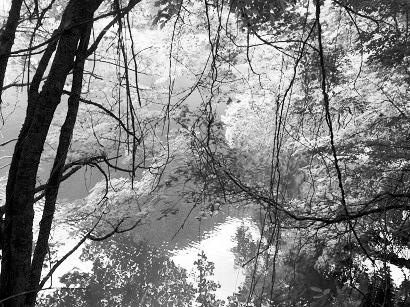
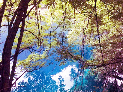
| original rgb image | grayscale image | grayscale equalized image |
|---|---|---|
| Independent histogram equalization based on color channel | Histogram equalization based on average value of color channel | Intensity component equalization based on HSI color space |
Histogram equalization usually increases the global contrast of many images, especially when the usable data of the image is represented by close contrast values. But it’s not the case to every image and different methods of processing color image matter a lot. Here’s some examples.
Here I am not showing the histogram but it’s the most useful and effective tool for analysis.
Case 1: Backgrounds and foregrounds are both bright or both dark
The method is useful in images with backgrounds and foregrounds that are both bright or both dark. In particular, the method can lead to better views of bone structure in x-ray images, and to better detail in photographs that are over or under-exposed. (wiki)
For this situation, the results usually have the following features.
| Method(Best to worst) | Effect | speed | Explaination |
|---|---|---|---|
| Histogram equalization based on average value of color channel | Higher saturation and better detail | Slowest | Considers the relevance of R, G and B channel. The change of luminance increases contrast and the changes of hue and saturation improve the color effect. |
| Intensity component equalization based on HSI color space | Darker and less detail | Medium | Applying equalization to the luminance increases contrast but not adjusting the hue and saturation weaks color in this case |
| Independent histogram equalization based on color channel | Changes in the image’s color balance. Greener/bluer in whole. | Fastest | Not considering the relevance of R, G and B channel but applying the same method on the Red, Green, and Blue components of an RGB image changes the relative distributions of the color channels |
Case 2: Backgrounds are brighter or darker
It also works well when applied to images with backgrounds much brighter or foregrounds much brighter.
In this typical case, the three methods of color image histogram equalization have the following effect.
| Method(Best to worst) | Effect | speed | Explaination |
|---|---|---|---|
| Intensity component equalization based on HSI color space | Brighter and higher saturation, less detail in some darken area | Medium | Apply equalization to the luminance only without resulting in changes to the hue and saturation of the image. |
| Histogram equalization based on average value of color channel | Brighter and better detail | Slowest | Considers the relevance of R, G and B channel. Because the equalization is based on the average histogram, the results’ color distributes more evenly without high saturation. The hue and saturation change as well. |
| Independent histogram equalization based on color channel | Changes in the image’s color balance. Greener/bluer in whole. | Fastest | Not considering the relevance of R, G and B channel but applying the same method on the Red, Green, and Blue components of an RGB image changes the relative distributions of the color channels |
Case 3: Good results for all methods
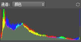
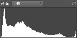
This is because the histograms of color channels and luminance channel have very similar distribution. Following are the rgb histogram and luminance histogram of original rgb image.
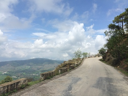
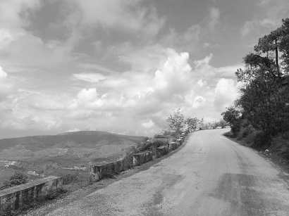
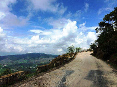
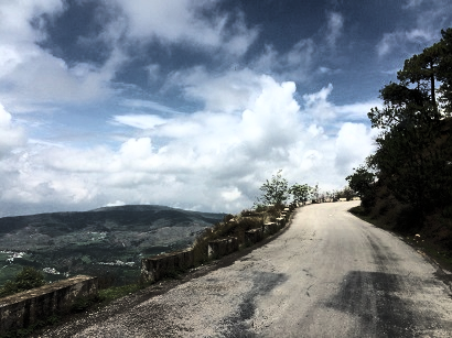
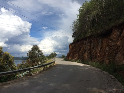
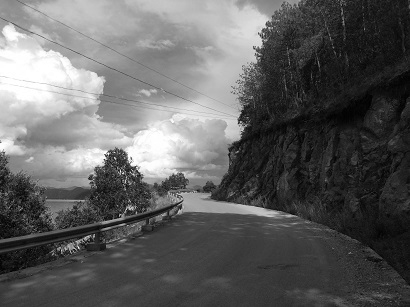
Case 4: Bad results for all methods
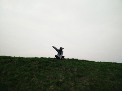
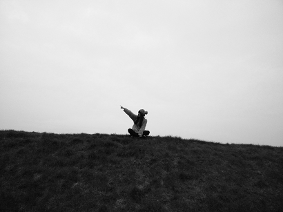
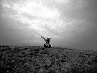
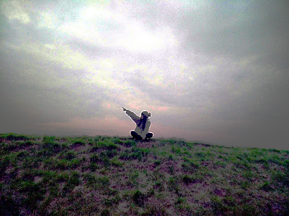
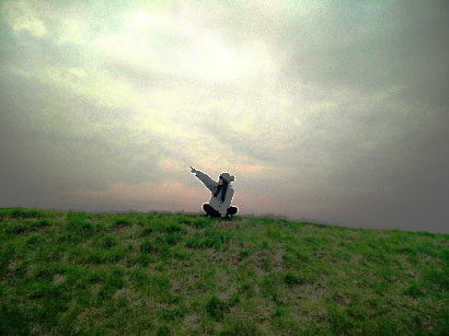
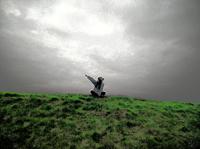
This group of results are bad. Let’s take a look at histogram.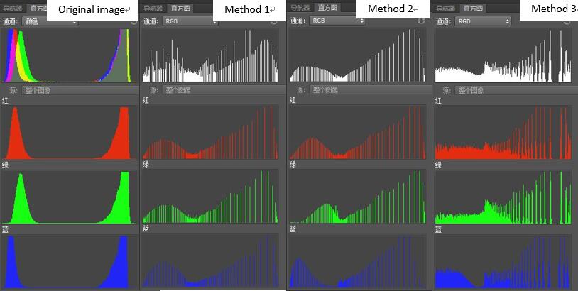
You can find out this image’s intensities concentrate in low(grasses) and high(sky) levels while seldom in medium(boundary) levels which is hard to spread out evenly.
But I am wondering why the figure will be outlined against the background with white line. Any ideas?