Automatically stiching several individual images to generate a panorama image.
Follow the routine described in the paper Automatic Panoramic Image Stitching using Invariant Features.
Theory and practice of panorama image stitching.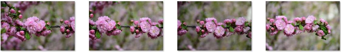

Credit: source images (flowers) comes from Example Data of OpenPano

Here’s the algorithm described in the paper: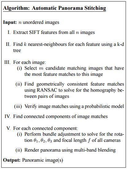

Algorithm

Extract SIFT Features

Idea of SIFT

Image content is transformed into local feature coordinates that are invariant to translation, rotation, scale, and other imaging parameters

Steps

I mainly follows the routine described in Tutorials of SIFT: Theory and Practice.

Constructing a scale space Ensure scale invariance.
Each octave’s image size is half the previous one. In each octave, progressively blur out images. By constructing a scale space, we express the image in different scale. In the following steps, all scales will be taken into consideration and the keypoint representation should be dependent of scales. Following are four octaves and each octave has five images.
LoG Approximations Fast approximation of Laplacian of Gaussian used to find keypoints.
The results of previous step are used to generate DOG(Difference of Gaussian). That is, the difference between two consecutive scales of each octave.

The Laplacian of Gaussian(LoG) operation is effective for finding edges and corners (usually keypoints) on the image. It goes like bluring and calculate second order derivatives. However, LoG is computationally expensive and is not scale invariant. DoG images are approximately equivalent to LoG images but faster.
Finding keypoints Locate maxima and minima in the Difference of Gaussian image.
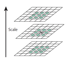
Iterate through each pixel and check its 26 neighbours (if any). In the following figure, X marks the current pixel. The green circles mark the neighbours. They distribute in three consecutive scales (one octave). Mark maxima and minima.

In practice, 5 level of blurs in each octave generates 5 Gaussian blurred images in each octave and will result in 4 DoG images. They can gernerate 2 extream images. Here’s the example image of that cat we used before.
Get rid of bad key points Edges and low contrast regions are bad keypoints.
Removing low contrast features: Select a threshold and reject those smaller value pixel. The value is the magnitude of the intensity at the current pixel in the DoG image (minima/maxima in previous step).
Removing edges: Edges are detected by two perpendicular gradients. An edge keypoint has one big gradient (perpendicular to the edge) and one small gradient (along the edge). When both gradients are small, the point is in a flat region. This case is also be rejected. We only accept keypoints in corners, where two gradients are both big.
Assigning an orientation to the keypoints Ensure rotation invariant.
Calculate gradient magnitudes and orientations for all points in the scale space.
$$m(x,y)=\sqrt { {(L(x+1,y)-L(x-1,y))}^2+{(L(x,y+1)-L(x,y-1))}^2 }$$
$$\theta {(x,y)}={tan}^{-1}((L(x,y+1)-L(x,y-1))/(L(x+1,y)-L(x-1,y)))$$
Then, an orientation histogram is used to store the orientation of keypoints and their neighbour regions. The peaks in the histogram correspond to dominant orientations.
Generate SIFT features A 128 dimensions vector is used to represent each keypoint.
A $16\times 16$ window around the keypoint is used to generate such distinctive feature.

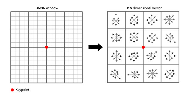
It’s composed of sixteen $4\times 4$ windows. Let’s focus on one $4\times 4$ window.

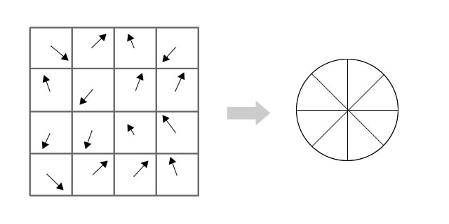
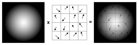
Each pixel/cell has a direction. Every sixteen directions are collected by an orientation histogram. Considering the pixels closer to keypoint (in the center) affect more than further pixels, we use a “gaussian weighting function” to assign different value. In the following figure, the farther away, the lesser the magnitude (darker).

Find k nearest-neighbours & Select Candidate Mating Images

In order to detect and stitch adjacent images, we need to match features. For every pair of image (a query image and a searched image), find 2 nearest-neighbours for each feature of query image in searched image using a k-d tree. If the best match much better than the next, accept. Then we can obtain some feature pairs for each pair of image. The size of feature pairs indicates in what degree this pair of image are matched (have similar features). A threshold is used to select m candidate matching images that have the most feature matches to this image.

RANSAC for estimating homography

RANSAC Idea

Random sample consensus (RANSAC) is an iterative method to estimate parameters of a mathematical model from a set of observed data that contains outliers, when outliers are to be accorded no influence on the values of the estimates. Therefore, it also can be interpreted as an outlier detection method. (wiki)

The features pairs we detected in previous may be noisy, we need to filter cleaner features.

Steps

I mainly follows the routine described in RANdom SAmple Consensus (slide by Aaron Bobick).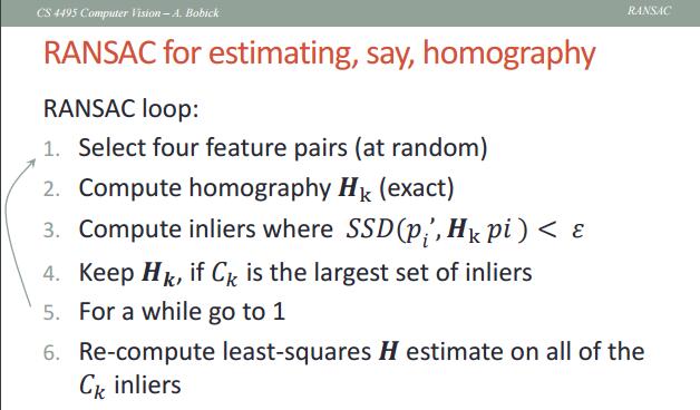

The loop iteration N is determined adaptively.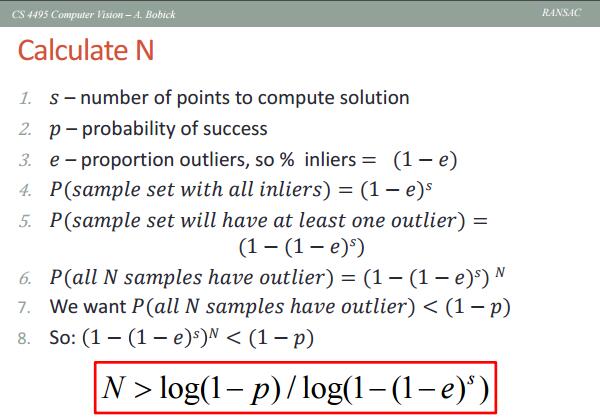

Then four feature pairs are selected randomly for computing homography, which is used to matching points for any two images taken from a camera at some fixed points.
For homography we have $x’=H \times x$ where $x’=[u_i,v_i]$ is a point in the reference image and $x=[x_i,y_i]$ is a point in the image that we want to warp. In order to calculate H we have to solve the following equation: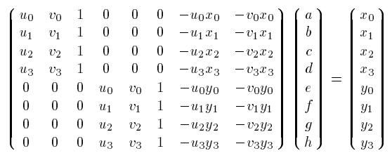

$$\begin{bmatrix}a && b && c \cr d && e && f \cr g && h && 1 \end{bmatrix}$$
Credit: Image Stitching Report By Ali Hajiabadi

Then, using the matrix H, warp one of the feature in each feature pairs and calculate the Sum of Square Differences (SSD) with the other feature. If the SSD is small enough (smaller than threshold), then the keypoints of this feature pair is considered as inliers.
Record the H relating to largest set of inliers and re-compute least-squares H estimate on all of those inliers.

Mlti-band blending

Idea

The idea behind multi-band blending is to blend low frequencies over a large spatial range, and high frequencies over a short range. [1]

Now we have detected adjacent images and warpped then for stitching. The next step is seamlessly stitch the overlapping area and blend them.

Steps

I mainly follows the routine described in Image Stitching II (slide by Linda Shapiro)

Forming a Gaussian Pyramid
- Start with the original image G0
- Perform a local Gaussian weighted averaging function in a neighborhood about each pixel, sampling so that the result is a reduced image of half the size in each dimension.
- Do this all the way up the pyramid Gl = REDUCE(Gl-1)
- Each level l node will represent a weighted average of a subarray of level l.
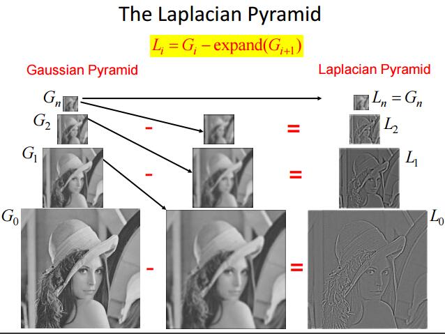
Compute Laplacian pyramid of images and mask: Making the Laplacians Li=Gi-expand(Gi+1)
- subtract each level of the pyramid from the next lower one
- EXPAND: interpolate new samples between those of a given image to make it big enough to subtract
Create blended image at each level of pyramid: Forming the New Pyramid
- A third Laplacian pyramid LS is constructed by copying nodes from the left half of LA to the corresponding nodes of LS and nodes from the right half of LB to the right half of LS.
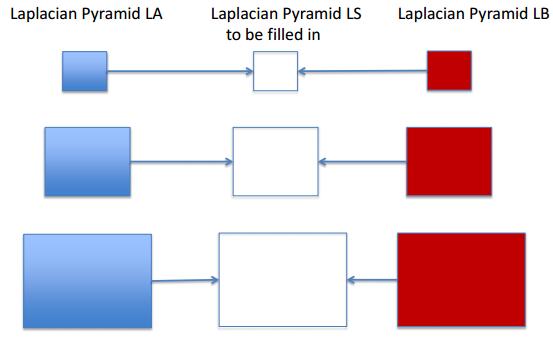
- Nodes along the center line are set equal to the average of corresponding LA and LB nodes
Reconstruct complete image: Using the new Laplacian Pyramid
Use the new Laplacian pyramid with the reverse of how it was created to create a Gaussian pyramid. Gi=Li+expand(Gi+1) The lowest level of the new Gaussian pyramid gives the final result.

Implementation

Implement with The CImg Library and VLFeat open source library in C++ language. Test on Visual Studio 2015, C++11. Images should be of bmp format(much easier to convert by ImageMagick).
My codes reference to AmazingZhen/ImageStitching since it’s compact, without too much dependencies, writing from scratch and satisfying basic requirements. My sincere thanks! Just because its effect is not very good in blending and has bugs especially in stitching many (~10) images, I have space to improve it in many perspectives. Currently, my codes is not robust but neat and easy to understand. I should futher work on this project. If looking for more complete and robust codes, I recommend OpenPano: Automatic Panorama Stitching From Scratch.

Source codes and images can be found here. Everything is well explained (hope so) in the code with comments, so I am not going to paste codes here. Any feedback is welcomed!

Usage of VLFeat

Download and unpack the latest VLFeat binary distribution (currently VLFeat 0.9.20 binary package) in a directory of your choice (e.g. F:\vlfeat-0.9.20-bin)
For Mac users, read this Apple X-Code tutorial.
These instructions show how to setup a basic VLFeat project with Visual Studio 2015 on Windows 10 (64 bit). Instructions for other versions of Visual Studio and Windows should be similar.

Specify the value of the PATH environment variable. E.g. Add F:\vlfeat-0.9.20-bin\vlfeat-0.9.20\bin\win64 to Path, where win64 depends on your architecture.
Open VS and select File > New > Project and choose General > Empty Project.
Click Project > Properties to open Property Pages. Choose Configuration > All Configurations.
Select Configuration Properties > C/C++ > General and add the root path of the VLFeat folder (e.g. F:\vlfeat-0.9.20-bin\vlfeat-0.9.20) to Additional Include Directories.
Select Configuration Properties > Linker > General and add the bin/win32 folder (even if your architecture is win64) (e.g. F:\vlfeat-0.9.20-bin\vlfeat-0.9.20\bin\win32) to Additional Library Directories.
Select Configuration Properties > Linker > Input and add vl.lib to Additional Dependencies.
Copy the vl.dll file in bin/win32 folder (e.g. F:\vlfeat-0.9.20-bin\vlfeat-0.9.20\bin\win32) to your VS project’s debug or release folder (e.g. C:\Users\HYPJUDY\Documents\Visual Studio 2015\Projects\PanoramaImageStitching\Debug).
Build and run the project (Ctrl+F5)

Reference: Using from C and Microsoft Visual Studio tutorial.

Results and Analysis

Source images: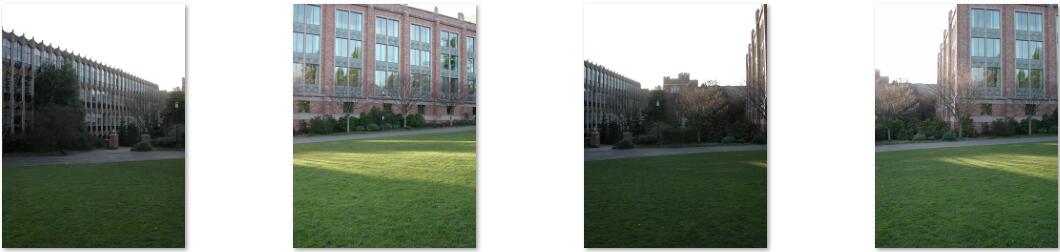

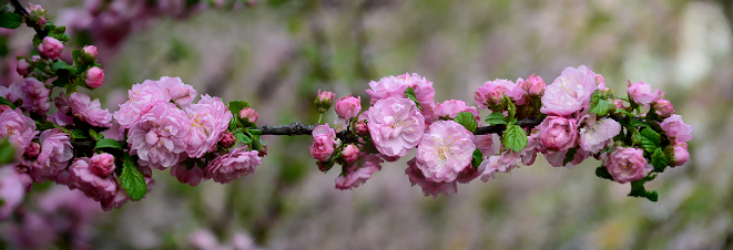
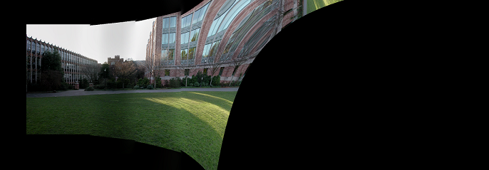
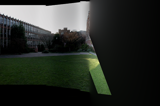
Result: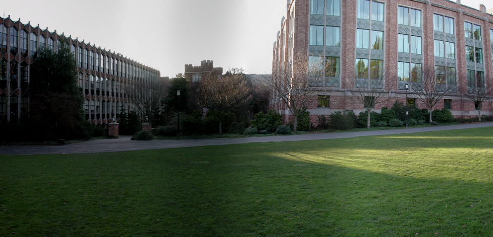

The above image is cropped. Before cropping, you can easily identify the warpped images.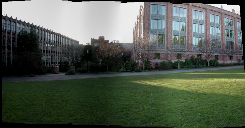

You should also have noticed that the warpped images have cylinder surfaces. The step of warpping images by a cylindrical or spherical projection can effective improve results’ quality. Following is the stitched image without cylidrical projection, which has vertical distortion. Find more about cylindrical panoramas at this page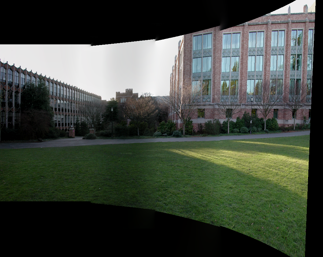

Notice that in the RANSAC for estimating homography procedure, since four feature pairs are selected randomly for computing homography, we may obtain different results each run. Some results can be very bad due to one or several images’ distortion.

The reason is the number of inliers is used as criteria for calculating homography transformation matrix H. “However, for high-resolution images, it’s common that you’ll actually find false matches with a considerable number of inliers, as long as enough RANSAC iterations are performed.”[5] Thus, after each matrix estimation, we should perform match validation check. I skip this part in my code currently and thus have a high chance of getting distorted stitched image when the number of source images is large.

Reference & Futher Reading

Paper: Automatic Panoramic Image Stitching using Invariant Features
Tutorials of SIFT: Theory and Practice by Utkarsh Sinha and corresponding code with OpenCV
k-d Tree Introduction (in chinese)
RANdom SAmple Consensus (slide by Aaron Bobick)
OpenPano: Automatic Panorama Stitching From Scratch and post OpenPano: How to write a Panorama Stitcher
VLFeat open source library
Image Stitching Report By Ali Hajiabadi
Image Stitching II (slide by Linda Shapiro) and Image Stitching
Cylindrical Panoramas
Slide: Automatic Image Alignment
Slide: Homographies and Mosaics
Image Alignment and Stitching: A Tutorial by Richard Szeliski
Wiki: Random sample consensus
Wiki: Scale-invariant feature transform
YouTube video: Microsoft Photosynth
Panoramas Assignments from Washington CSE 576, Spring 2017 (c++ skeleton code provided, use Harris corner detector); Berkeley CS194-26
Reports by Riyaz Faizullabhoy, by Japheth Wong from CS194-26 courses.