A caffe version implementation of a hash network(DNNH/NINH) for similarity-based visual research based on paper: Hanjiang Lai, Yan Pan, Ye Liu, and Shuicheng Yan. Simultaneous feature learning and hash coding with deep neural networks, CVPR 2015.

Assume $I$ to be the image space. The goal of hash learning for images is to learn a mapping $F:I->{0,1}^q$, such that an input image $I$ can be encoded into a q-bit binary code $F(I)$, with the similarities of images being preserved.

Motivation

Image Retrieval

Extracting informative image features —— Deep Convolutional Neural Network: extract discriminative features depend on data, build end-to-end relation between the raw image data and the binary hashing codes
Learning effective approximate hashing functions —— Hash Code => efficiency
- Space-saving: high-dimensional features to lower dimensional space, compact bitwise representation
- Speedup: binary pattern matching or Hamming distance measurement

Approaches

These learning-based approaches usually comprise two stages:

Projecting the high dimensional features onto the lower dimensional space.
Quantizing the generated real-valued representations into binary codes.

Three building blocks of DNNH

A shared sub-network with a stack of convolution layers to produce the effective intermediate image features;
- Basic framwork: Network in Network, insert convolution layers with $1\times 1$ filters after some convolution layers with filters of a larger receptive field. use an average pooling layer as the output layer.
- Parameter sharing: this sub-network is shared by the three images in each input triplet. Significantly reduce the number of parameters.
  
  Click me for an explict diagram of each layer in browser.
A divide-and-encode module to divide the intermediate image features into multiple branches, each encoded into one hash bit;
- Divide the input intermediate features into q slices with equal length. Then each slice is mapped to one dimension by a fully-connected layer, followed by a sigmoid activation function that restricts the output value in the range $[0, 1]$ and a piece-wise threshold function to encourage the output of binary hash bits. After that, the q output hash bits are concatenated to be a q-bit (approximate) code.
- Trying to reduce the redundancy among the hash bits: each hash bit is generated from a separated slice of features.
A triplet ranking loss designed to characterize that one image is more similar to the second image than to the third one.
- Preserve relative similarities of the form “image $I$ is more similar to image $I^+$ than to image $I^-$”.
- More easily to obtained than pairwise similarities (e.g. the click-through data from image retrieval systems)
- From paper: Triplet ranking hinge loss is defined by
  $$
  \begin{equation}
  \begin{split}
  & \hat l_{triplet}(F(I),F(I^+),F(I^-))\\
  & =max(0,1-(\left\lVert F(I)-F(I^-) \right\rVert_H-\left\lVert F(I)-F(I^+) \right\rVert_H)), \\
  & s.t. F(I),F(I^+),F(I^-)\in \{0,1\}^q
  \end{split}
  \end{equation}
  $$
  where $\left\lVert .\right\rVert_H$ represents the Hamming distance. For ease of optimization, natural relaxation tricks are to replace the Hamming norm with the $l_2$ norm and replace the integer constraints on $F(.)$ with the range constraints. The modified loss functions(used in forward propagation in neural networks) is
  $$
  \begin{equation}
  \begin{split}
  & \hat l_{triplet}(F(I),F(I^+),F(I^-))\\
  & =max(0,\left\lVert F(I)-F(I^+) \right\rVert_2^2-\left\lVert F(I)-F(I^-) \right\rVert_2^2+1), \\
  & s.t. F(I),F(I^+),F(I^-)\in[0,1]^q
  \end{split}
  \end{equation}
  $$
  
  This variant of triplet ranking loss is convex. Its (sub-)gradients(used in backward propagation in neural networks) with respect to $F(I)$, $F(I^+)$ or $F(I^-)$ are
  $$
  \begin{equation}
  \begin{split}
  & \frac {\partial l}{\partial b} =(2b^–2b^+)\times I_{||b-b^+||_2^2-||b-b^-||_2^2+1>0}\\
  & \frac {\partial l}{\partial b} =(2b^+-2b)\times I_{||b-b^+||_2^2-||b-b^-||_2^2+1>0}\\
  & \frac {\partial l}{\partial b} =(2b^–2b)\times I_{||b-b^+||_2^2-||b-b^-||_2^2+1>0}
  \end{split}
  \end{equation}
  $$
  where we denote $F(I)$, $F(I^+)$ or $F(I^-)$ as $b$, $b^+$ or $b^-$. The indicator function $I_{condition}=1$ if $condition$ is true; otherwise $I_{condition}=0$.

Image Retrieval and Evaluation of DNNH

In image retrieval procedure, an image X is first encoded into k-dimension feature in the forward pass of pretrained model. Then, a quantization operation is exploited to generate hash codes.

Given a query image, the retrieval list of images is produced by sorting the hamming distances between the query image and images in search pool. The performance can be evaluated by metric of mean average precision(MAP). (Also see chinese version explaination)
Details in Implementation part.

Implementation

Architecture of DNNH

To do: Write prototxt to define DNNH and bash files to execute for training on preprocessed triplet CIFAR-10 dataset.

Overview and Structure of Dataset

We start with a data layer that reads from the LevalDB database we created earlier. Each entry in this database contains the image data for a triplet of images. In order to pack a triplet of images into the same blob in the database we pack one image per three channels(RGB). That is to say, for triplet train/validation images, each entry has 9 channels of I, I+ and I- respectively. Pool and query images also have 9 channels in each entry except that 3 images in 9 channels are the same.
In training phase, since the input of triplet ranking hinge loss layer here should be I, I+ and I-, we want to be able to work with these three images separately while at the same time share the parameters between layers on three sides (the sub-network is shared by the three images in each input triplet). This can be done by firstly adding a slice layer after the data layer to slice input data along the channel dimension and secondly naming the same parameters to share parameters between layers.
In testing phase, only one side is needed and loss layer should be delete.

Above is the architecture of my 12-bit hash code DNNH(caffe-dnnh/runtime/12bit/train12.prototxt) drawn by netscope editor. Click me(training phase) or me(testing phase) for an explict diagram of each layer in browser. Read codes and also see this weight sharing example for more details.

Attention: We use dropout, an effective and simple regularization technique in neural networks. It should only be used in training phase but not testing/predicting phase. The reason why you can find dropout layer in my caffe prototxt for testing is the operation is implemented by if (this->phase_ == TRAIN) condition and inverted dropout. Read code CAFFE-ROOT/src/caffe/layers/dropout_layer.cpp for more details.

Triplet ranking hinge loss layer

Loss drives learning by comparing an output to a target and assigning cost to minimize. The loss itself is computed by the forward pass and the gradient w.r.t. to the loss is computed by the backward pass.(Caffe Loss Layer)

Init in function LayerSetUp, Forward_cpu and Backward_cpu are direct implementation of the two formulas we mentioned above.

The Solver optimizes a model by first calling forward to yield the output and loss, then calling backward to generate the gradient of the model, and then incorporating the gradient into a weight update that attempts to minimize the loss. (Forward and Backward)

Also see: Developing new layers in Caffe.

Image Retrieval and Model Evaluate

To do: Write prototxt to encode images and bash files to execute for image retrieval. Implement the metric of mean average precision (mAP) for evaluation.
In image retrieval task, we can employ one hashing stream in the DNNH architecture to generate k-bit hash codes for each input image. In this procedure, an image X is first encoded into k-dimension feature in the forward pass of pretrained model. Then, a quantization operationis exploited to generate hash codes. Do this procedure with query images and pool images, here I get the approxiamate hash codes output in caffe.cpp and write the result hashcode into files and read them out when I need to calculate MAP.

Hamming distance

The Hamming distance between two strings of equal length is the number of positions at which the corresponding symbols are different.(wiki)

Wiki gives us a neat implementation on C, which takes use of fast bitwise XOR(exclusive or). It also uses an algorithm of Wegner (1960) that repeatedly finds and clears the lowest-order nonzero bit.

int hamming_distance(unsigned x, unsigned y)
{
    int dist = 0;
    unsigned  val = x ^ y;
    while (val != 0) { // Count the number of bits set
        // A bit is set, so increment the count and clear the bit
        dist++;
        val &= val - 1;
    }
    return dist; // Return the number of differing bits
}

But this implementation limits to binary integers input which is insuffcient for us (e.g. 24-bit, 48-bit). Thus I use string type as follow. Input x and y can have different length and the shorter one will be padded with zero prefix.

int hamming_distance(string x, string y) {
    int dist = 0;
    int i = x.size() - 1, j = y.size() - 1;
    for(i, j; i >= 0 && j >= 0; --i, --j) { 
        if(x[i] != y[i]) ++dist;
    }
    while(i != -1) {
      if(x[i--]) ++dist;
    }
    while(j != -1) {
      if(y[j--]) ++dist;
    }
    return dist;
}

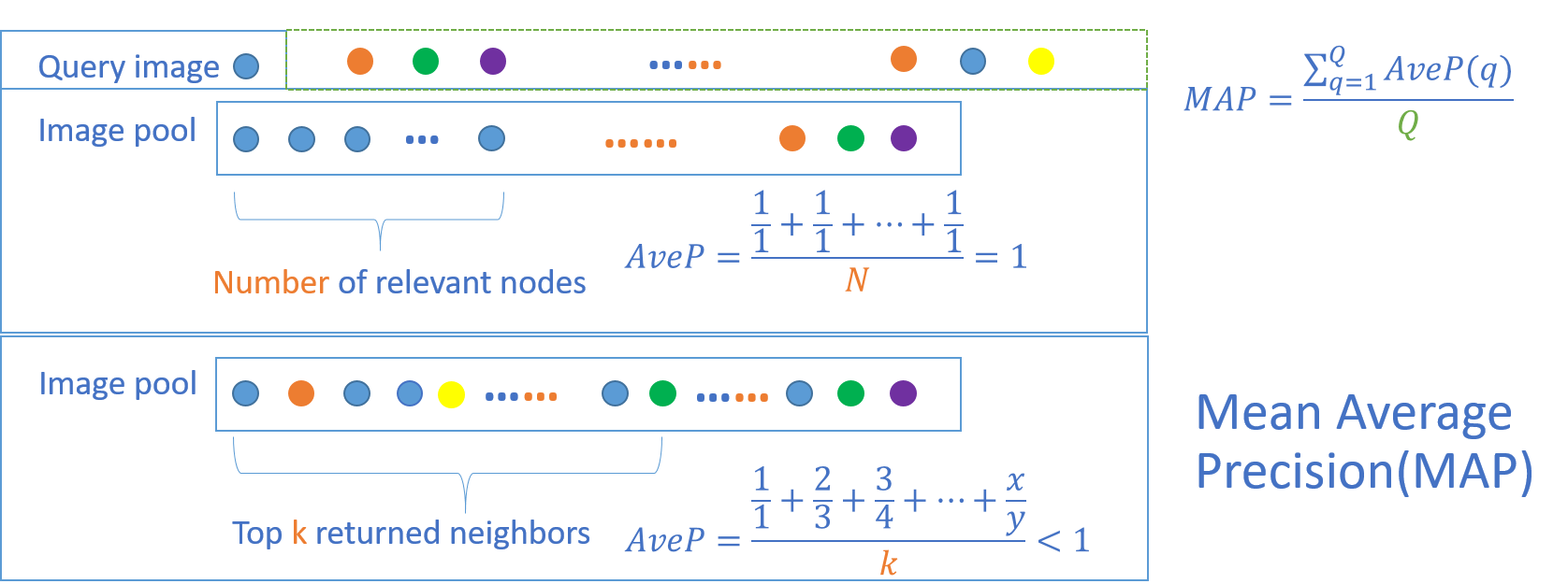
Metric of Mean Average Precision (mAP)

Mean average precision for a set of queries is the mean of the average precision scores for each query.
$$MAP=\frac {\sum _{q=1}^{Q} AveP(q) }{Q}$$
$$AveP=\frac {\sum _{k=1}^{n} (P(k)\times rel(k))}{number\ of\ relevant\ documents}$$
where Q is the number of queries and $rel(k)$ is an indicator function equaling 1 if the item at rank $k$ is a relevant document, zero otherwise. Note that the average is over all relevant documents and the relevant documents not retrieved get a precision score of zero.(wiki)

Here we can modify the formula to calculate the MAP values within the top k returned neighbors. The denominator of MAP take the smaller one of k and number of relevant images. And the numerator of MAP should be the average of the precision at cut-off k in the retrieval list. I also calculate the MAP respect to 10 labels in CIFAR-10 dataset respectively.

Results and Analysis

To do: Draw performances for 12-bit, 24-bit and 48-bit hash code and make some analysis.

Different lengths of hash codes

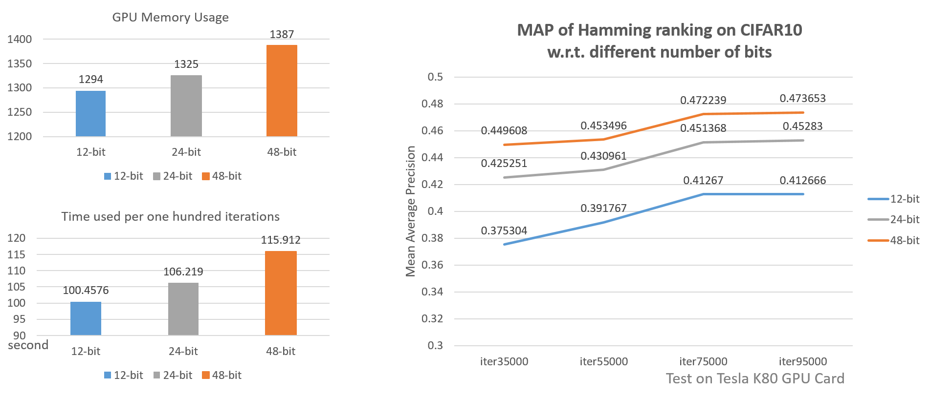
We can clearly see from the above diagram that shorter codes have the edge in space and time usage while longer codes have higher accuracy. But will 128-bit codes have much higher accuracy? Maybe not. Because if shorter codes are capable of presenting images then large bits may be overfitting.

Different labels

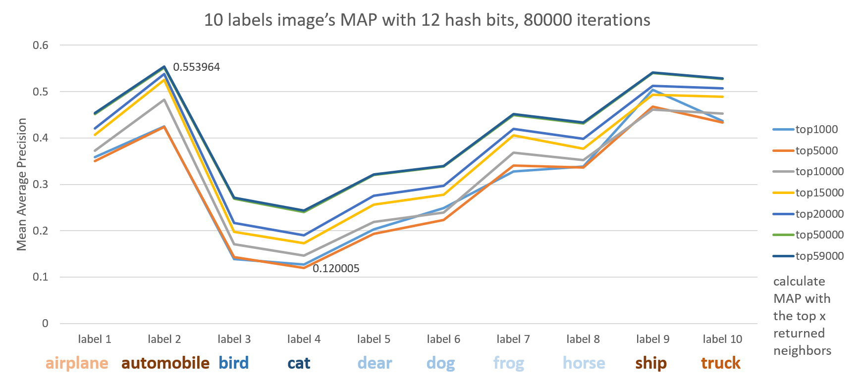
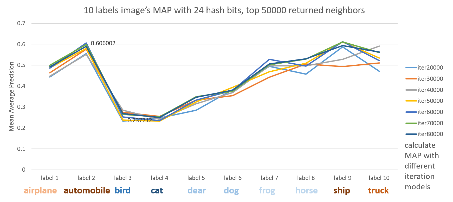
Here we see artifacts like automobile, ship, truck, airplane outperform animals like cat, bird, dear dog and so on.

Further Improvements

From the above results we can infer that MAP closely relates to labels/classes in the CIFAR-10 dataset. A first thought is to treat different labels differently and focus more on images with lower MAP labels. Since the margin in triplet hinge loss function characterizes the difference of similarity between dissimilar pair of image and similar pair of image, we can design different margins for different labels/classes. More specifically, larger margins for artifacts and smaller margin for animals.
$$
\begin{equation}
\begin{split}
& \hat l_{triplet}(F(I),F(I^+),F(I^-))\\
& =max(0,margin-(\left\lVert F(I)-F(I^-) \right\rVert_H-\left\lVert F(I)-F(I^+) \right\rVert_H)), \\
& s.t. F(I),F(I^+),F(I^-)\in \{0,1\}^q
\end{split}
\end{equation}
$$
Inspired by Fine-tuning CaffeNet, since CIFAR-10 dataset is small and training from scratch takes much time, I think we can try to use fine-tune on pre-trained deep models for better performance in both speed and precision.
How about four images a group? For example: $\{F(I^{a,b}),F(I^a),F(I^b),F(I^-)\}$. $F(I^{a,b})$ is image with tag $a$ and $b$, $F(I^a)$ and $F(I^b)$ are images with tag $a$ and $b$ respectively while $F(I^-)$ neither has tag $a$ or $b$. Because one image may contains several tags, this design aims to preserve semantic similarity as well.

[Caffe] Similarity-Based Deep Neural Network Hashing